
Introduction
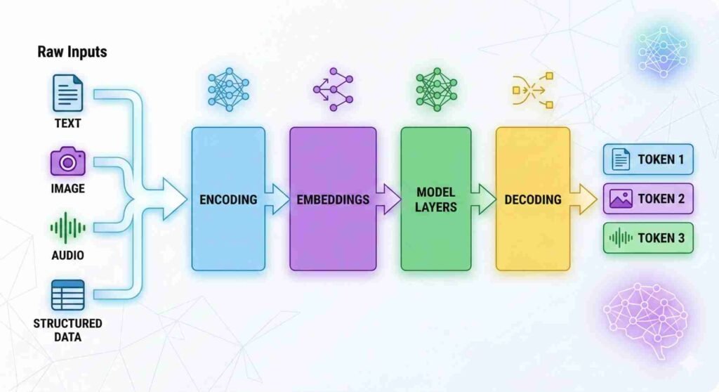
How AI tools transform raw data during inference is central to understanding how output is generated. In AI systems, “raw data” refers to unprocessed input presented in human-interpretable form, such as text strings, images composed of pixel values, audio waveforms, or structured numerical records. Although these inputs appear meaningful to users, they are not directly processed in their original format.
During the inference process in AI tools, the system converts incoming input into numerical representations that can be evaluated by stored parameter configurations. This transformation occurs within a predefined computational architecture composed of the core structural components of AI tools and does not involve modification of model weights. The distinction between training and inference stages, including why runtime prompts do not alter stored parameters, is examined in our analysis of the training–inference boundary in AI tools.
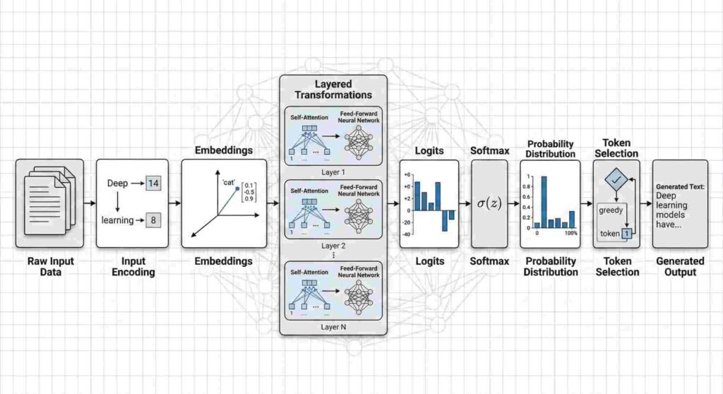
The output generated by an AI tool is therefore the result of structured internal processing applied to encoded input representations. This transformation typically proceeds through a sequence of stages including input encoding, embedding representation, layered computational transformations, probability computation, and output decoding, where numerical operations are applied to data within the model’s representational space.
How AI Tools Transform Raw Data During Inference
In deployed systems, input arrives in formats designed for human interpretation rather than direct computational processing. Although users perceive text, images, audio, or structured records as meaningful content, models operate on numerical representations derived from those inputs.
Text as Tokens
For text-based systems, raw input consists of character sequences. Before processing, the text is segmented into tokens. Tokens may represent full words, subword units, or character fragments depending on the tokenization scheme used during model development. Each token is mapped to a numerical identifier, which enables subsequent retrieval of learned vector representations.
The model does not process sentences as semantic wholes; it evaluates numerical token sequences within its representational framework.
Images as Pixel Tensors
Image inputs are represented as multi-dimensional arrays of pixel intensity values. Each image is encoded as a tensor containing numerical values corresponding to color channels and spatial coordinates. The model operates on these numerical tensors rather than the visual scene as perceived by a human observer.
Audio as Waveform Signals
Audio input is typically captured as waveform signals represented by sequences of numerical amplitude values over time. These signals are often transformed into frequency-domain representations, such as spectrograms, to facilitate structured numerical analysis within the model architecture.
Structured Data as Numerical Arrays
Tabular or structured datasets may already contain numerical values, but they still require standardized formatting. Categorical fields may be encoded into numeric form, and numerical fields may be normalized or scaled to align with model expectations. The resulting data is organized into arrays or tensors for computation.
Across modalities, the defining principle remains consistent: AI systems do not process human-readable input directly. All input must first be converted into numerical structures compatible with the model’s internal computational layers.
Stage 1: Input Encoding
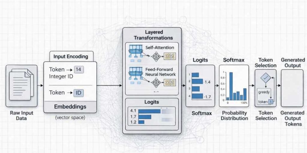
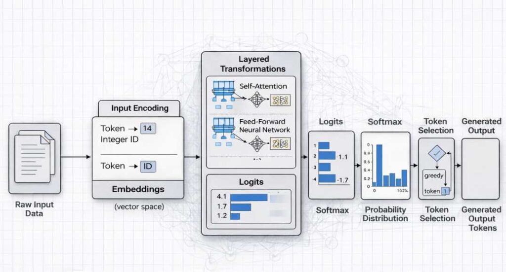
Input encoding refers to the conversion of externally provided data into numerical representations that can be processed by a model’s internal computational layers. AI systems operate on tensors and vectorized data structures; therefore, human-readable inputs must first be transformed into structured numerical form.
Tokenization in Text Models
In text-based systems, raw character strings are segmented into smaller units called tokens. Tokens may represent whole words, subword fragments, or individual characters depending on the model’s vocabulary design.
Each token is then mapped to a corresponding integer index within a predefined vocabulary. This indexed sequence forms the basis for subsequent embedding and transformation operations.
Patch Embedding in Vision Models
In image-processing systems, visual input consists of pixel arrays. These arrays are typically divided into fixed-size patches or regions. Each patch is flattened and projected into a numerical vector space through learned linear transformations.
This patch-based representation enables image data to be processed using the same vector-based computational mechanisms applied in other model architectures.
Spectrogram Transformation in Audio Models
Audio signals are continuous waveforms. To facilitate structured processing, the waveform is transformed into a time–frequency representation, commonly a spectrogram.
The spectrogram converts amplitude variations across time into a two-dimensional numerical representation that captures frequency components. This structured matrix format allows subsequent computational layers to operate on discrete numerical features.
Feature Normalization
Across modalities, numerical inputs may undergo normalization procedures. These include scaling values to standardized ranges, centering distributions, or adjusting variance.
Normalization ensures that encoded inputs conform to the numerical assumptions embedded in the model’s parameter configuration, enabling consistent downstream computation.
Stage 2: Embedding Representation
Learned Embedding Matrices
After initial encoding converts raw input into discrete tokens or numerical features, the system transforms these units into continuous vector representations. This transformation is performed using learned embedding matrices that are stored as part of the model’s trained parameter set.
An embedding matrix maps each discrete input unit (such as a token identifier) to a dense numerical vector of fixed dimensionality. If a model uses a 768-dimensional embedding space, each token is represented as a vector containing 768 numerical values. These values are learned during the training phase through parameter optimization rather than manually assigned.
Vector Dimensionality
The dimensionality of the embedding space determines the representational capacity available to encode statistical relationships between input elements. A higher-dimensional space allows more parameters to capture relational structure, although dimensionality alone does not determine model behavior.
Embedding vectors function as coordinates within a structured representational space shaped by training data and optimization procedures. The relative positioning of vectors reflects statistical co-occurrence patterns encoded during training.
Positional Encoding in Sequence Models
In sequence-based architectures, positional encoding is applied to preserve order information. Embedding vectors alone do not encode token position. Therefore, an additional positional representation is combined with token embeddings.
In transformer-based systems, positional encodings may be implemented as learned parameters or deterministic functions that assign each position a vector component. This enables the model to distinguish identical tokens appearing in different sequence locations.
Representational Space Placement
The combined embedding and positional representation places each input element within a high-dimensional representational space. Tokens that share statistical context during training tend to occupy neighboring regions within this space.
The geometry of this space reflects distributed representation learning principles described in foundational literature (Goodfellow, Bengio & Courville, 2016; Bishop, 2006). Relationships between tokens are encoded through learned parameter configurations rather than explicit symbolic rules.
Fixed Parameters During Inference
It is important to clarify that embedding matrices remain fixed during inference. The mapping from token to vector is determined by stored parameters learned during training. When new input is processed, the system retrieves and applies these predefined vectors without modifying the embedding structure.
Embedding representation therefore functions as the bridge between discrete symbolic input and continuous numerical computation. All subsequent transformations operate on these vectorized representations within the learned parameter-defined space.
Stage 3: Layered Transformations
After input encoding and embedding, the numerical representation progresses through multiple computational layers within a model architecture organized into functional layers. These layers apply structured mathematical transformations that gradually reshape the input representation into a form suitable for output prediction.
Weighted Matrix Multiplication
At the core of most neural network architectures is weighted matrix multiplication. Each layer contains parameter matrices learned during training. During inference, the embedded input vector is multiplied by these matrices.
This operation performs a linear transformation, projecting the representation into a new coordinate space. The weights determine how features are amplified, suppressed, or combined.
Nonlinear Activation
Following linear transformation, a nonlinear activation function is applied element-wise to the resulting vector. Common activation functions include ReLU, GELU, and sigmoid functions, depending on architecture.
Nonlinear activation enables the model to represent complex relationships that cannot be captured through linear transformation alone. Without nonlinearity, stacked matrix multiplications would collapse into a single linear transformation.
Activation functions modify intermediate numerical states but do not alter stored parameters.
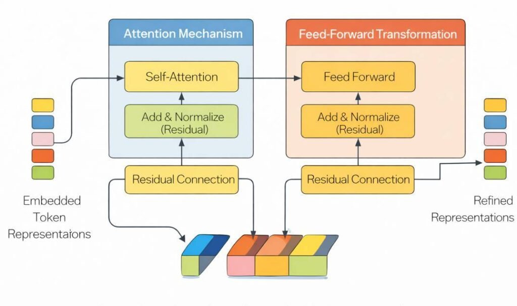
Attention Mechanisms (in Many Modern Systems)
In transformer-based architectures, layered transformations include attention mechanisms. Attention computes weighted relationships between elements of a sequence.
Each token representation is compared with others using learned projection matrices to produce query, key, and value vectors. These are used to calculate attention scores that determine how information from different positions influences the current representation.
Attention modifies how contextual information is distributed across the sequence but operates using fixed parameter weights during inference.
Residual Connections
Many modern architectures incorporate residual connections. These connections add the original input of a layer to its transformed output before passing it forward.
Residual pathways support representational stability across deep networks. They allow gradient signals to propagate effectively during training and preserve information during inference.
Residual addition modifies the intermediate activation state but does not update model parameters.
Layer Stacking
These transformations are repeated across multiple layers. Each layer incrementally refines the internal representation, progressively shaping it toward a distribution that supports probability computation in the final stage.
Across all layered transformations, the system applies fixed learned parameters to the input representation. The internal state evolves numerically within a fixed parameter configuration.
Stage 4: Probability Computation
After layered transformations are applied to encoded input representations, the model produces a numerical vector commonly referred to as logits.
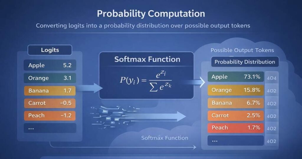
Logits
Logits are unnormalized numerical scores assigned to each possible output token (or class, depending on the model type). These values are generated by applying a final linear transformation to the model’s internal activation state.
Logits do not represent probabilities.
They are real-valued scores that indicate relative preference before normalization.
Higher logit values correspond to stronger internal activation for a given token relative to others in the vocabulary.
Softmax Normalization
To convert logits into a probability distribution, most language models apply the softmax function.
The softmax function:
- Exponentiates each logit value
- Normalizes the result by dividing by the sum of all exponentiated logits
- Produces a vector of values between 0 and 1
- Ensures the total probability sums to 1
The result is a probability distribution over all possible next tokens.
At this stage, the model has not “chosen” an output. It has computed a structured distribution reflecting learned statistical relationships encoded in its parameters.
Distribution Over Outputs
This normalized vector represents the model’s evaluation of possible continuations given the current input context.
For a vocabulary-based language model, this distribution may contain tens of thousands of possible tokens. Each token is assigned a probability reflecting its relative compatibility with the preceding sequence.
The distribution is recalculated at each generation step, conditioned on previously generated tokens.
Probability Concentration and Output Reliability
In many cases, probability values are concentrated among a small subset of candidate tokens.
However, the distribution may also be spread across a large number of tokens with similar probability values.
When probability mass is distributed broadly rather than concentrated on a small set of candidates, the model may produce outputs that do not correspond to verified factual information. These outputs arise from statistical continuation patterns encoded during training rather than from direct retrieval of validated knowledge.
The probability distribution therefore reflects statistical compatibility with the input context, not factual verification.
Deterministic vs Stochastic Decoding
Once probabilities are computed, a decoding strategy determines how the next token is selected.
Deterministic decoding selects the token with the highest probability at each step.
This approach produces consistent outputs for identical inputs.
Stochastic decoding samples from the probability distribution.
Sampling strategies may include:
- Temperature scaling (adjusting distribution sharpness)
- Top-k sampling (restricting selection to the k highest-probability tokens)
- Nucleus (top-p) sampling (restricting to tokens whose cumulative probability exceeds a threshold)
In deterministic decoding, output selection is fixed by the highest probability value.
In stochastic decoding, variability arises from probabilistic sampling across eligible tokens.
The difference lies in how the computed probability distribution is used during token selection.
Stage 5: Decoding and Output Rendering
After probability computation, the model produces a distribution over possible next elements in the sequence. These elements may represent tokens in text systems, pixel segments in image systems, or structured outputs in other modalities.
Token Selection
From the computed probability distribution, one candidate element is selected. Selection may occur through:
- Deterministic methods (e.g., choosing the highest-probability token)
- Stochastic sampling methods (e.g., temperature scaling, top-k, or nucleus sampling)
The selection process operates strictly on the probability distribution produced during the forward pass.
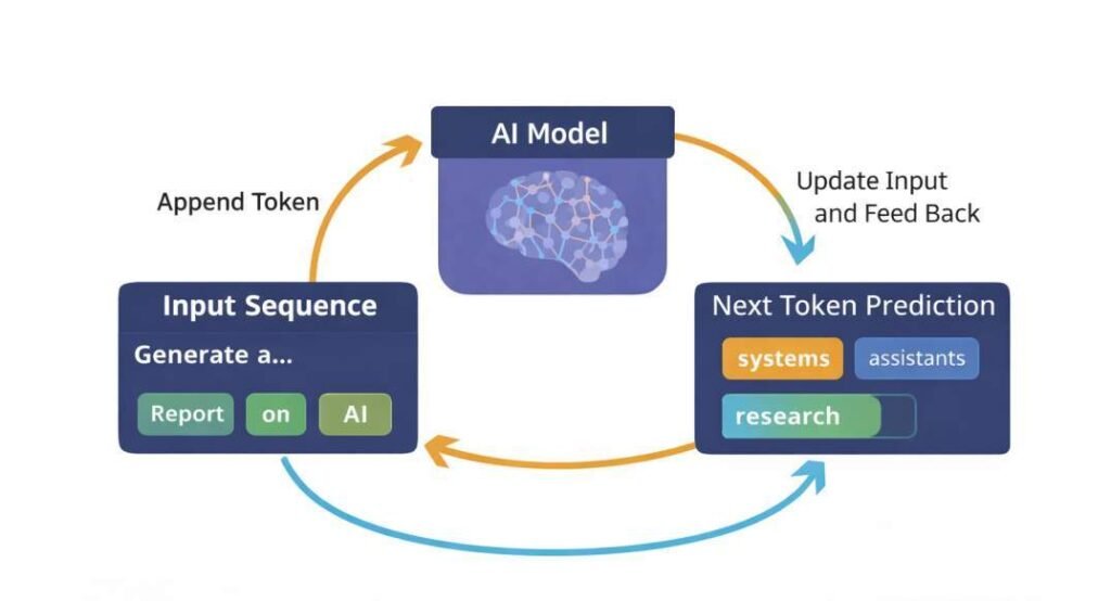
Sequential Generation
In autoregressive systems, output is generated iteratively. After one token is selected, it is appended to the input context and passed back through the model to compute the next probability distribution. This process repeats until a termination condition is met (such as an end-of-sequence marker or length limit).
Each iteration reuses the same model configuration. Internal activation states change temporarily across steps, but the parameter configuration remains fixed.
Rendering into Human-Readable Form
Selected tokens are converted from their internal numerical representations back into readable format:
- Token IDs are mapped to text strings
- Subword units are merged
- Formatting rules are applied
In image or audio systems, decoded numerical outputs are transformed back into pixel arrays or waveform signals.
This rendering stage converts numerical output into externally interpretable form. It does not introduce new information into the model’s stored parameters.
Structural Clarification
Decoding and rendering are procedural steps that transform computed probabilities into usable outputs. They do not involve gradient computation, dataset integration, or parameter updates. Learning mechanisms operate exclusively during training, not during output generation. At this point, the full transformation from raw input to structured output has been completed without modification to stored model parameters.
Internal State vs Stored Parameters During Inference
This section reinforces the training–inference boundary established earlier without restating the full analysis.
In deployed operation, AI systems generate output through temporary internal activation states that arise as input data moves through computational layers. These activation states represent intermediate numerical transformations produced at each stage of processing. They are dynamic and exist only for the duration of the current input sequence.
Stored parameters, by contrast, are the learned weight values established during the training phase. These parameters define how inputs are transformed at each layer of the model. During deployment, they remain fixed and are not modified by individual user interactions.
While stored parameters remain unchanged, the model conditions each new prediction on the sequence of tokens currently present in the input context window. This temporary contextual information influences internal activation patterns during processing but does not modify the model’s stored parameter weights.
It is important to distinguish between:
- Internal state: transient activation values generated while processing a specific input.
- Stored parameters: persistent weight matrices learned during model training.
Changes in output across different prompts reflect differences in activation patterns within a fixed parameter structure, not structural modification of the model itself.
The architectural separation between internal state and stored parameters has been examined in a separate analysis. Why AI Tools Don’t Learn From Your Prompts (Training vs Input Data). That distinction remains central to understanding how transformation pipelines operate during inference.
Architectural Variations in AI Data Transformation
While many modern AI tools follow a similar high-level processing pipeline—encoding, transformation, and output computation—the internal transformation mechanisms vary across architectural families.
Transformer-Based Systems
Transformer architectures are widely used in contemporary language and multimodal models. These systems process input through attention mechanisms that compute relationships between elements in a sequence.
Instead of relying solely on fixed positional progression, transformers evaluate contextual relationships by calculating weighted interactions across tokens or input segments. This enables the system to represent long-range dependencies within encoded data.
Layered self-attention operations and feed-forward transformations progressively refine internal representations before probability computation.
Convolutional Systems
Convolutional architectures are commonly applied to spatial data such as images. These systems use convolutional filters to detect localized patterns within structured input grids.
Rather than computing relationships across all positions simultaneously, convolutional layers apply learned kernels across neighboring regions. This allows hierarchical feature extraction, where lower layers detect simple patterns and deeper layers combine them into more complex structures.
The transformation process remains parameter-defined and deterministic during inference.
Recurrent Systems
Recurrent architectures process sequential input step-by-step, maintaining an internal state that updates as new elements are received.
Instead of evaluating all input positions simultaneously, recurrent systems propagate information forward through time, updating a hidden state that summarizes prior elements in the sequence.
Although internal state evolves during processing, stored parameters remain fixed during inference.
Structural Commonality Across Architectures
Despite differences in internal computation mechanisms—attention-based, convolutional, or recurrent—all architectures follow the same fundamental transformation principle:
- Input is encoded into numerical representation.
- Stored parameters apply structured mathematical transformations.
- Internal activations evolve temporarily.
- Output probabilities are computed within the same stored parameter structure.
Architectural variation changes how transformation occurs, but not the training–inference boundary established in prior discussion.
Why This Structural Distinction Matters
Understanding the transformation pipeline clarifies that AI systems do not modify stored parameters during individual interactions. Output variation across prompts reflects differences in temporary activation states within a fixed parameter structure. Recognizing this boundary helps prevent misconceptions about runtime learning or adaptive memory during inference. This sequence explains how AI tools transform raw data into structured numerical representations before output rendering.
Conclusion
AI-generated output is produced through a sequence of internal computational transformations applied to encoded input data. Raw inputs are first converted into numerical representations, positioned within learned embedding spaces, and processed through layered mathematical operations defined by stored parameter weights.
These operations generate probability distributions over possible outputs, from which final responses are decoded and rendered into human-readable form. Throughout this process, parameter configurations remain unchanged.
References
Bishop, C. M. (2006). Pattern Recognition and Machine Learning. Springer.
Goodfellow, I., Bengio, Y., & Courville, A. (2016). Deep Learning. MIT Press.
Available at: https://www.deeplearningbook.org/
Vaswani, A., et al. (2017). Attention Is All You Need. Advances in Neural Information Processing Systems (NeurIPS).
https://arxiv.org/abs/1706.03762
Rumelhart, D. E., Hinton, G. E., & Williams, R. J. (1986). Learning representations by back-propagating errors. Nature, 323, 533–536.